Thunderstorms in Poland, 2014 edition
 Marcin Polkowski
Translated from Polish. Originally published on morony.pl on 14 Sep 2016.
At the end of 2013 I had the idea of regularly saving an image (a map) showing the current locations of lightning strikes. At the time I was using the blide.de website. Of course I had no intention of doing it by hand, so I set up a script on a server that saved the current image every 15 minutes on the dot. The script is still running and keeps saving the latest maps. I remembered it when the server started running out of disk space. I downloaded the images to my computer and started playing. First up was the first full year – 2014.
In theory, over 365 days I should have saved 365*24*4 = 35040 images. In practice I saved 34999, which is pretty good. The first, obvious thought was an animation. I combined all the images into a video:
In the next step I wanted to approach the subject more thoroughly. How do you estimate the number of strikes on each map? The number itself can't be estimated, of course, but the area covered by storms can. On the maps, red marks places where at least one strike occurred in the last 15 minutes. Unfortunately the files are saved as heavily compressed jpg, but you can clearly see what's red and what isn't. I quickly hacked together a script in Matlab:
clear;clc
files=dir('2014/blids/*.png');
S = zeros(length(files), 2);
for a = 1:length(files)
    name = ['2014/blids/' files(a).name];
    C = strsplit(name, '/');
    C2 = strsplit(C{end},'.');
    date = C2{1};
    time = C2{2};
    I = imread(name);
    idx = (I(:,:,1)>100 & I(:,:,2)<100 & I(:,:,3)<100);
    S(a,1) = sum(sum(idx));
    S(a,2) = datenum(str2double(date(1:4)), str2double(date(5:6)), str2double(date(7:8)), str2double(time(1:2)), str2double(time(3:4)), 0);

    fprintf('%d\t%d\n',a,S(a,1));
end
For each map, the script calculated and saved the number of pixels where strikes occurred. Now all that's left is to put it nicely on a plot: for example, summed up for each day.
clf
days = datenum(2014,01,01):datenum(2014,12,31);
storm = zeros(size(days));

for d = 1:length(days)
    storm(d) = sum(S(S(:,2)>=days(d)&S(:,2)<days(d)+1,1));
end
%storm(storm>0)=log10(storm(storm>0));
stairs(days-datenum(2014,01,01),storm, 'LineWidth',2)
axis([0 365 0 2.5e5])
hold on
for month = 1:12
    plot(ones(1,2)*datenum(2014,month,1)-datenum(2014,01,01),[0 2.5e5], 'k--')
end
And here's the result: 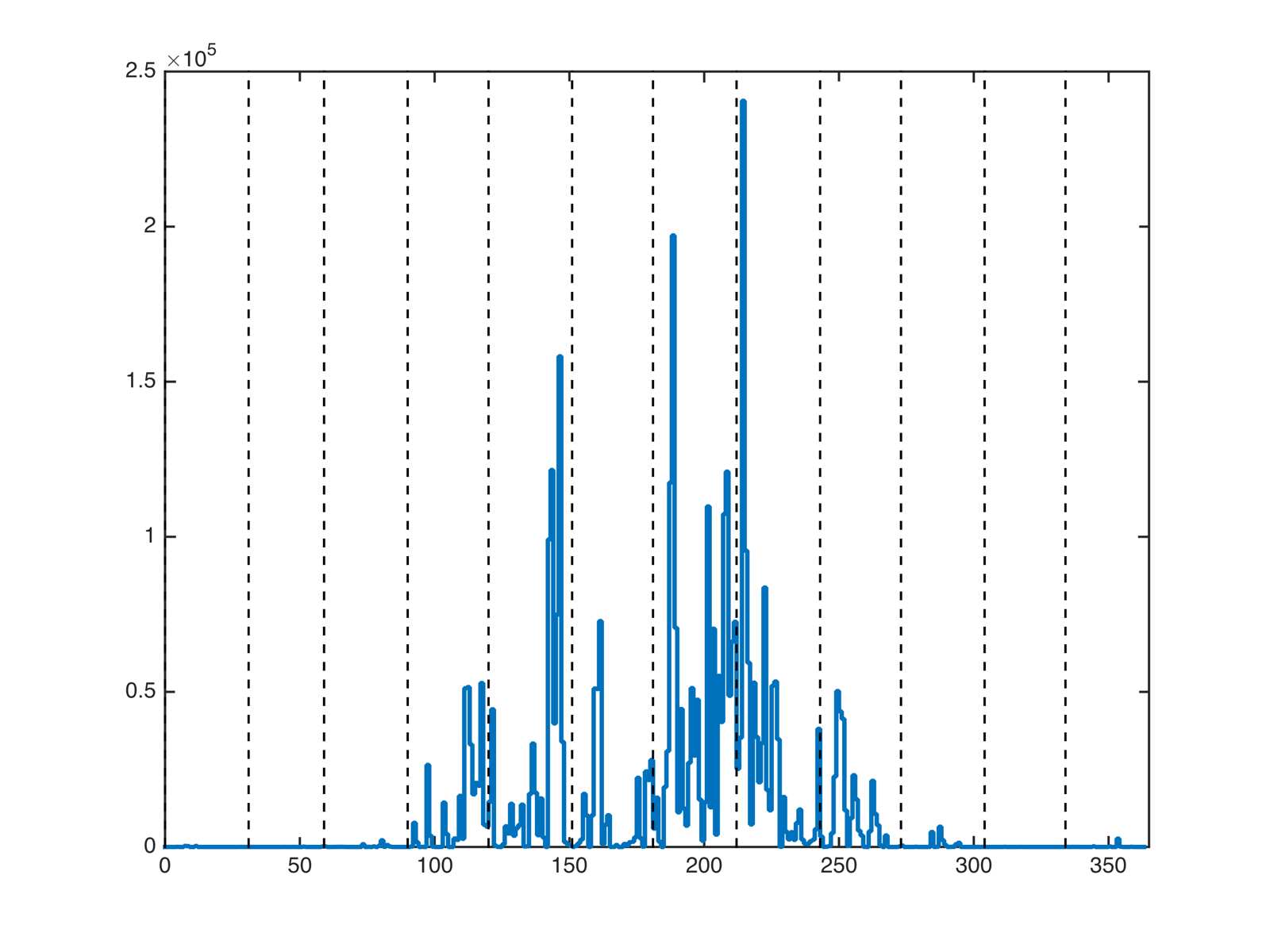
The vertical lines separate the months. You can see increased thunderstorm activity from April to September. The peak falls at the beginning of August, which you can also see in the video.
How would you use data like this? When I have a spare moment, I'll make an animation and a plot for 2015.