The effect of seasonal ionosphere changes on GPS measurements
 Marcin Polkowski
Translated from Polish. Originally published on morony.pl on 21 Sep 2016.
For four years I've been taking part in the passive seismic experiment "13BB star". I'll be writing about it many more times, but I need a couple of sentences of introduction here. The goal of the experiment is to record natural seismic events, which makes it possible to map deep structures in the Earth. As part of the experiment, 13 standalone stations hidden deep in the forests were operating in Pomerania. Each station was equipped with a GPS receiver, whose job was to provide very precise timing information. On the side, and more or less incidentally, once an hour each station also logged its GPS position: longitude, latitude and height above sea level.
One day I decided to load this data for one of the stations into Matlab. When I plotted the measured height above sea level against time, a barely visible seasonal change caught my interest. The scatter of ±10 meters in the measurements is no surprise at all, since "civilian" GPS measurements (as opposed to survey-grade ones) come with roughly that kind of error. What intrigued me was the seasonal shift in the measurements, which is very clearly visible once you plot a weekly moving average: 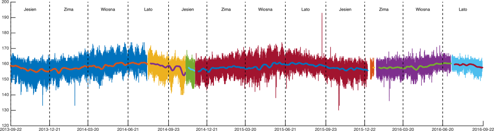
I immediately checked whether a similar effect shows up at the other stations: 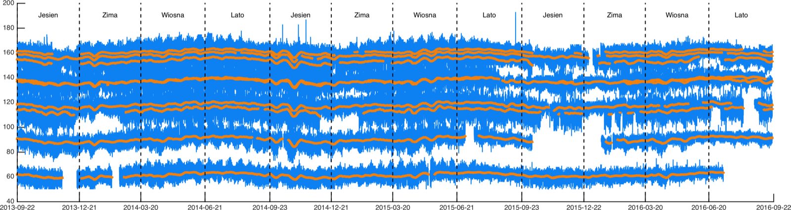
It gets even more interesting when you compare the moving averages for all the stations by subtracting the mean over the whole period. Below are the 7-day averages: 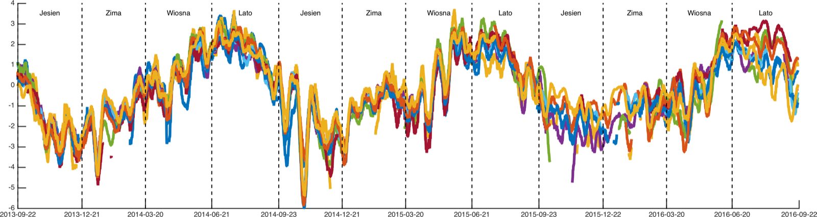
30-day: 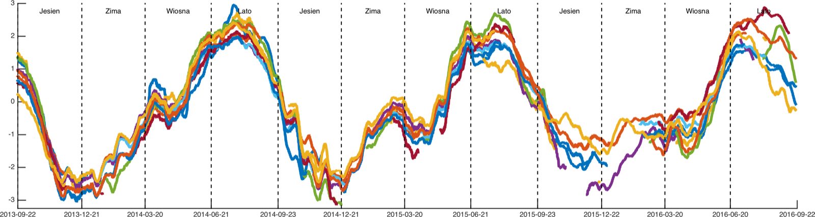
and 60-day: 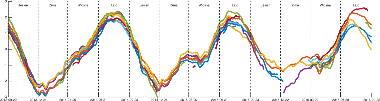
The plots above show a clear seasonality in the changes. I asked a specialist in GPS reference measurements for a comment: "ionosphere, standard stuff, boring". What I find interesting, though, is that if the effect is so well known and so repeatable, why hasn't a correction been introduced for it? It's precisely the dynamics of ionospheric changes that limits the accuracy of civilian GPS. Survey equipment uses permanent reference stations, which make it possible to determine the effect of the ionosphere on the measurement at a given moment (a permanent station doesn't move, so any deviation in its measurement comes from changes in the ionosphere). Such rapid local changes can't be predicted, but the changes between summer and winter seem entirely repeatable and obvious.
In case anyone is interested in the code used to generate the bottom 3 figures:
%% 7 days
clf; hold on
files = dir('*.gps');

colors = lines(length(files));

for fi = 1:length(files)
    X = load(files(fi).name);
    D = X(:,1) - circshift(X(:,1),[1 0]);
    idx = [1; find(D>1); length(X(:,1))]; % Find gaps in the data longer than 1 day
    X(X(:,4)>500,4)=NaN;
    X(X(:,4)<50,4)=NaN; % Remove off-the-wall measurements
    for a = 1:length(idx)-1
        i = idx(a):idx(a+1)-1;
        i(isnan(X(i,4)))=[];
        f = nanmean(X(:,4)); % Mean over the whole period
        if length(i) > 7*24 % Only look at segments longer than 7 days
            % Compute and plot the moving average, shifted by the global mean
            plot(X(i,1), tsmovavg(X(i,4),'s',7*24,1)-f, 'Color', colors(fi,:), 'LineWidth',3)
        end
    end
end

% Plotting and dividing the figure into seasons

axis([datenum(2013,09,01) datenum(2016,07,31), -6 4])
pory = [datenum(2013,09,22) datenum(2013,12,21) datenum(2014,03,20) datenum(2014,06,21) datenum(2014,09,23)  datenum(2014,12,21) datenum(2015,03,20) datenum(2015,06,21) datenum(2015,09,23) datenum(2015,12,22)  datenum(2016,03,20) datenum(2016,06,20) datenum(2016,09,22)];

names = {'Wiosna', 'Lato', 'Jesien', 'Zima'};
for a = 1:length(pory)-1
    text(mean(pory(a:a+1)),3.5,names{rem(a+1,4)+1},'HorizontalAlignment', 'Center', 'FontSize', 15);
    plot([pory(a) pory(a)], [-10 10],'k--')
end

set(gca,'xTick', pory)

datetick('x','YYYY-mm-dd','keepticks')

hgexport(gcf, '13BB_GPS_003_7.png', hgexport('factorystyle'), 'Format', 'png', 'resolution', 300, 'Width', 40, 'Height', 10);