Smog armageddon
 Marcin Polkowski
Translated from Polish. Originally published on morony.pl on 11 Jan 2017.
Over the last few days the media have been dominated by the terrible air quality in Polish cities. This is not some abstract problem – all you have to do is step outside to see and smell how bad the air is. Smog needs two ingredients. The first is the production of harmful dust and pollutants, which is much higher in winter because of the heating season, especially from individual central heating systems with solid-fuel furnaces (wood, coal), often burning waste. Combined heat and power plants, even though they burn coal, emit proportionally less pollution per kW of energy thanks to the filters installed in them. The second condition necessary for smog to form is a temperature inversion layer in the atmosphere, which blocks the exchange of air near the ground with the air above the inversion boundary. If the inversion layer is at a height of 100-200 meters, we're sitting in a closed "jar" into which we're emitting huge amounts of pollution. So much for the short version of the theory; let's move on to practice.
Taking advantage of the very high dust concentration in Warsaw, I decided to check what the problem looks like from above. I managed to take two very telling shots:


The photo on the left shows the chimneys of the Siekierki combined heat and power plant with Warsaw's skyscrapers in the background. The photo on the right is a view of central Warsaw from near the Gdański Bridge. Unfortunately, what the photos show isn't clouds but the pollution we were forced to breathe.
At the same time, I started measuring dust concentration in the air outside my house in Legionowo. I bought a laser sensor and connected it to a Raspberry Pi. The sensor hangs right outside the window and talks to the Pi over a serial interface:
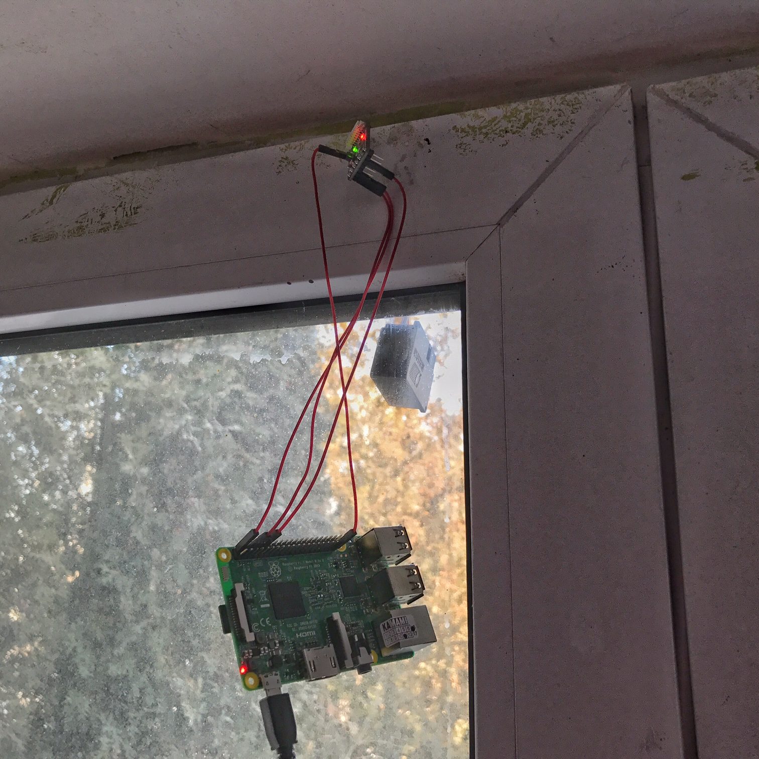
Each measurement gives three results corresponding to different dust fractions, including the "most popular" one, PM2.5. The program that receives the measurements is written in Python:
import serial
from time import gmtime, strftime

port = serial.Serial("/dev/serial0", baudrate=9600, timeout=1.5)
data = port.read(32);

f = open("/home/pi/" + strftime("%Y-%m-%d", gmtime()) + ".txt", "a")
if ord(data[0]) == 66 and ord(data[1])==77:
    suma = 0
    for a in range(30):
        suma += ord(data[a])

    if suma == ord(data[30])*256+ord(data[31]):

        PM01 = str(ord(data[4])*256+ord(data[5]))
        PM25 = str(ord(data[6])*256+ord(data[7]))
        PM10 = str(ord(data[8])*256+ord(data[9]))
        str = strftime("%Y-%m-%d %H:%M:%S", gmtime()) + "\t" + PM01 + "\t" + PM25 + "\t" + PM10;
        f.write(str + "\n")
        print(str)

port.close()
f.close()
The code above runs every minute. The data are saved to a plain text file:
2017-01-09 20:43:02 185 470 729
2017-01-09 20:44:02 181 440 682
2017-01-09 20:45:02 175 460 701
2017-01-09 20:46:02 172 445 725
2017-01-09 20:47:02 175 448 680
2017-01-09 20:48:02 177 449 725
2017-01-09 20:49:02 170 450 754
2017-01-09 20:50:02 176 458 746
2017-01-09 20:51:02 165 441 733
2017-01-09 20:52:02 174 434 707
2017-01-09 20:53:02 170 451 715
2017-01-09 20:54:02 170 436 702
Then, every 15 minutes, a script runs that draws the plot. To make it easier to read, it plots moving averages of the measurements rather than the raw measurements:
import numpy
import ftplib
from ftplib import FTP
import sys
from matplotlib.dates import strpdate2num
from datetime import datetime, timedelta
import matplotlib

matplotlib.use('Agg')
import matplotlib.pyplot as plt
date = sys.argv[1];
X = numpy.loadtxt('/root/AIR/OLSZANKOWA50A/'+date+'.txt', delimiter='\t', dtype=object, converters={0: lambda x: datetime.strptime(x.decode("utf-8"), "%Y-%m-%d %H:%M:%S"), 1: numpy.float, 2: numpy.float, 3: numpy.float})

window = 900;
step = 60;
ts = min(X[:,0])
tss = datetime(ts.year, ts.month, ts.day)
t = tss;
te = t + timedelta(days=1)

T = []
PM01 = []
PM25 = []
PM10 = []
while t < te:
    t = t + timedelta(seconds=step)
    idx = numpy.logical_and(X[:,0] > (t - timedelta(seconds=window)), X[:,0] < (t + timedelta(seconds=window)))
    #print(t, sum(idx))
    T.append(t)
    if sum(idx) > 0:
        PM01.append(numpy.mean(X[idx,1]))
        PM25.append(numpy.mean(X[idx,2]))
        PM10.append(numpy.mean(X[idx,3]))
    else:
        PM01.append(numpy.nan)
        PM25.append(numpy.nan)
        PM10.append(numpy.nan)

x = []
label = []
for a in range(0,24,1):
    x.append(tss+timedelta(hours=a))
    if a%2 ==0:
        label.append((tss+timedelta(hours=a)).strftime('%H:%M:%S'))
    else:
        label.append('')

plt.figure(figsize=(20, 10))
plt.plot(T,PM01, 'b', lw=2, label='PM 1.00')
plt.plot(T,PM25, 'r', lw=4, label='PM 2.50')
plt.plot(T,PM10, 'g', lw=2, label='PM 10.0')
plt.xlabel('Time [UTC]')
plt.ylabel('ug/m3')
plt.legend(loc='upper left', shadow=True)
plt.xlim([ts, te])
plt.ylim([0, (numpy.ceil(max(PM10)/50)+1)*50])
plt.grid()
plt.title(date)
plt.xticks(x,label, rotation=0)
plt.savefig('/root/AIR/OLSZANKOWA50A/'+date+'.png',dpi=300)

File2Send = '/root/AIR/OLSZANKOWA50A/'+date+'.png'
Output_Directory = "/public_html/parking-legionowo.pl/AIR/"

ftp = FTP('***************')
ftp.login('***************', '***************')
file = open(File2Send, "rb")
ftp.cwd(Output_Directory)
ftp.storbinary('STOR ' +date+'.png', file)
print("STORing File now...")
ftp.quit()
file.close()
print("File transfered")
Once the plot is ready, it's saved to a PNG file and sent to a server, where you can watch the measurements as they come in.
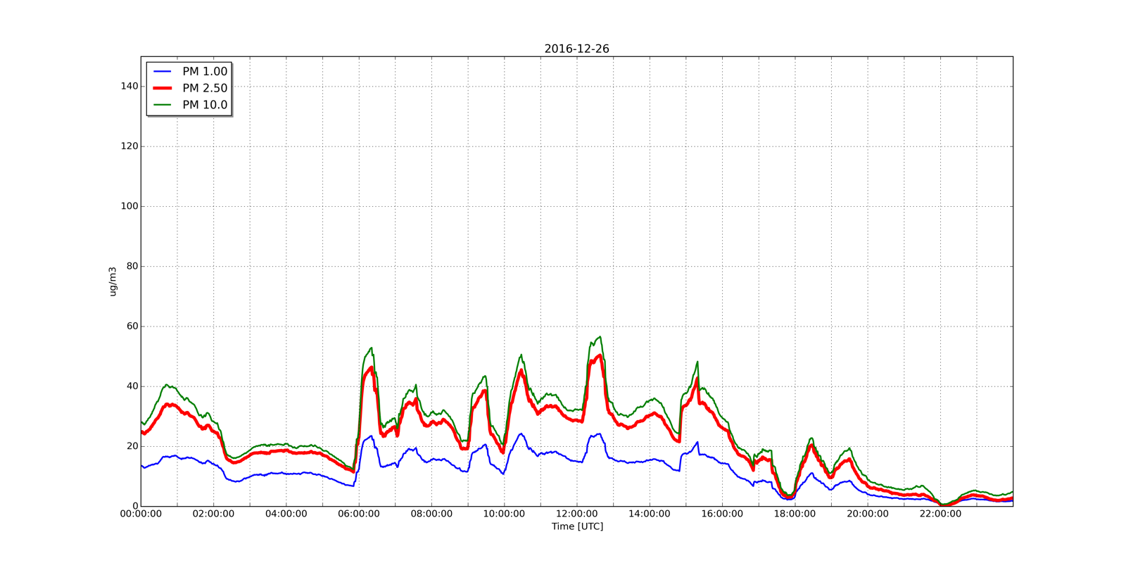
This is what a normal, "smog-free" day looks like (the brief spikes are probably the moments when the neighbors throw more coal into an old furnace):
And this is what a "smog" day looks like (that's when I took the photos shown at the beginning): 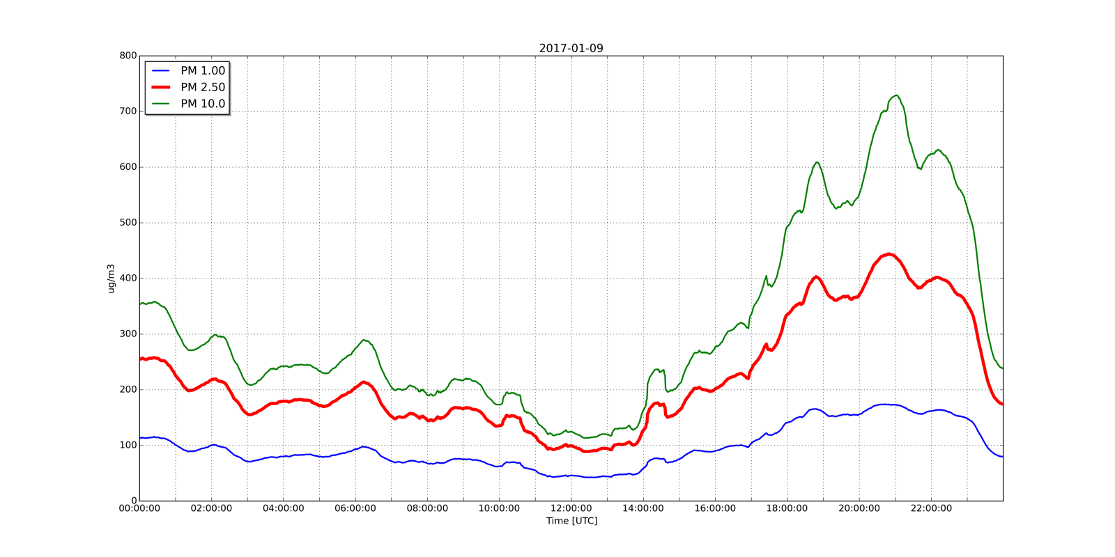
You can see the current measurements on the sponsor's website: http://parking-legionowo.pl/AIR/